A Practical Guide to Autonomous Trading Systems

A comprehensive introduction to designing, training, and deploying RL agents for systematic trading

---

Table of Contents

1. Introduction
2. What is a Trading RL Agent?
3. Why Reinforcement Learning for Trading?
4. Core Concepts You Need to Understand
5. The RL Trading Framework
6. Designing Your Trading Environment
7. Choosing Your RL Algorithm
8. The Training Process
9. Evaluation and Validation
10. Common Pitfalls and How to Avoid Them
11. Path to Production
12. Resources and Next Steps

---

Introduction

If you’re reading this, you’re probably fascinated by the idea of teaching a computer to trade autonomously. Maybe you’ve tried manual trading and found the emotional rollercoaster exhausting. Maybe you’re a developer who wants to apply machine learning to financial markets. Or maybe you’re a systematic trader looking to automate decision-making.

Here’s the truth upfront: Building a profitable trading RL agent is hard. It requires knowledge of trading, programming, machine learning, and financial markets. Most attempts fail. But when it works, it’s transformative.

This guide will give you the conceptual foundation to build your first trading RL agent. We won’t dive into code yet (that comes in Part 2), but by the end of this article, you’ll understand:

• What an RL agent actually is and how it differs from other trading systems
• The key components required to build one
• Common mistakes that cause most projects to fail
• A realistic path from concept to production

Let’s start with the fundamentals.

---

What is a Trading RL Agent?

Definition

A Reinforcement Learning (RL) Agent for trading is a computer program that learns to make trading decisions (buy, sell, hold) by interacting with a simulated market environment, receiving rewards for profitable actions and penalties for losses.

Unlike traditional algorithmic trading systems that follow hardcoded rules (“if RSI < 30, buy”), an RL agent discovers optimal trading strategies through trial and error, similar to how a human learns through experience.

Key Characteristics

1. Autonomous Decision Making

• The agent decides when to enter and exit trades
• No human intervention required once trained
• Adapts to changing market conditions

2. Learning from Experience

• Improves through repeated interactions with market data
• Learns from both successes and failures
• Can discover non-obvious patterns

3. Goal-Oriented

• Optimizes for specific objectives (profit, Sharpe ratio, drawdown control)
• Balances exploration (trying new strategies) with exploitation (using what works)
• Considers long-term consequences, not just immediate gains

4. Probabilistic

• Doesn’t guarantee profits on every trade
• Aims for positive expected value over many trades
• Manages uncertainty inherent in markets

What Makes RL Different?

Traditional Algorithmic Trading:

Human designs rules → Code implements rules → System executes
Example: "Buy when 50-day MA crosses above 200-day MA"

Machine Learning Trading:

Human selects features → ML model finds patterns → System predicts
Example: "Given these 50 features, predict next day's return"

Reinforcement Learning Trading:

Human designs environment → Agent explores strategies → Agent optimizes actions
Example: "Find the sequence of buy/sell/hold actions that maximize long-term profit"

The critical difference: RL agents learn strategy, not just prediction.

---

Why Reinforcement Learning for Trading?

The Case For RL

1. Handles Sequential Decision Making

Trading isn’t about predicting the next price—it’s about making a sequence of decisions:

• When to enter a position
• How much to risk
• When to scale in/out
• When to exit
• Whether to wait for better opportunities

RL is specifically designed for sequential decision problems. Each action affects future states and opportunities.

2. Optimizes for Your Actual Goal

Traditional ML models predict prices or returns. But that’s not your goal—your goal is profit.

RL agents optimize directly for what you care about:

• Total profit
• Risk-adjusted returns (Sharpe ratio)
• Maximum drawdown control
• Win rate and R-multiples

3. Considers Trade-offs

Should you take profit now or hold for a bigger move? Should you enter this marginal setup or wait for A+ confluence?

RL agents learn these trade-offs through experience, balancing:

• Immediate rewards vs. long-term value
• Certainty of small gains vs. uncertainty of large ones
• Risk of loss vs. opportunity cost of inaction

4. Adapts to Market Regimes

Markets change. What worked in 2020 might not work in 2025. RL agents can:

• Detect regime changes through environment feedback
• Adjust behavior in different conditions
• Continue learning from new data (with proper safeguards)

The Case Against RL (Why Most Fail)

1. Extreme Difficulty

Building a profitable RL trading agent requires expertise in:

• Financial markets (order flow, market structure, trading mechanics)
• Machine learning (model architecture, training, validation)
• Software engineering (robust infrastructure, data pipelines)
• Risk management (position sizing, drawdown control, failure modes)

Missing any one of these usually leads to failure.

2. Data Requirements

RL agents need vast amounts of training data:

• Historical price data (tick, 1-min, 5-min bars)
• Volume and order flow data
• Multiple market conditions (trending, ranging, volatile)
• Multiple instruments for robustness

With insufficient data, agents overfit and fail in live trading.

3. Training Instability

RL training is notoriously unstable:

• Agents can “forget” good strategies during training
• Hyperparameters are sensitive and hard to tune
• Reward function design is critical and non-obvious
• No guarantee of convergence to a good policy

Many projects train for weeks only to produce agents that lose money.

4. Overfitting is Easy

An agent might discover a strategy that works perfectly in backtests but fails live because:

• It exploited random patterns in historical data
• Training data doesn’t include current market conditions
• The strategy is too complex to generalize
• Transaction costs or slippage weren’t modeled correctly

5. Black Box Concerns

Unlike rule-based systems, you often can’t explain WHY an RL agent makes certain decisions:

• Hard to debug when it fails
• Difficult to gain confidence in the strategy
• Challenging to meet regulatory requirements
• Risk of unexpected behavior in edge cases

So Should You Still Try?

Yes, if:

• You have strong foundational trading knowledge (proven profitable manually or with systematic strategies)
• You’re proficient in Python and ML frameworks (TensorFlow, PyTorch, Stable-Baselines3)
• You have quality historical data or can acquire it
• You’re willing to invest 6-12 months learning and experimenting
• You understand this might not work, and that’s OK (learning is valuable)

No, if:

• You’re looking for a “get rich quick” automated money printer
• You have limited trading or programming experience
• You expect it to work within a few weeks
• You can’t tolerate the possibility of losing money while learning

The realistic path: Start with simple manual trading → Build rule-based systems → Add ML predictions → Finally attempt RL agents.

RL is the advanced final boss, not the starting point.

---

Core Concepts You Need to Understand

Before building an RL trading agent, you need solid understanding of these concepts:

1. The RL Framework (MDP)

RL problems are modeled as Markov Decision Processes (MDPs) with five components:

State (S):

• The agent’s observation of the world at time t
• In trading: current price, indicators, position size, P&L, time of day
• Example: [current_price, RSI, MACD, position, unrealized_PnL, bars_in_trade]

Action (A):

• What the agent can do
• In trading: typically [Buy, Sell, Hold] or [Long, Short, Flat, Scale_In, Scale_Out]
• Agent chooses one action per timestep

Reward (R):

• Immediate feedback for taking action A in state S
• In trading: could be profit/loss, Sharpe ratio, or custom metric
• Example: reward = realized_PnL - penalty_for_drawdown

Transition Dynamics (P):

• How the state changes after taking an action
• In markets: new bar arrives, position updates, P&L changes
• Usually stochastic (random/uncertain)

Policy (π):

• The agent’s strategy: mapping from states to actions
• What we’re trying to learn through RL
• Example: “In state S, take action A with probability p”

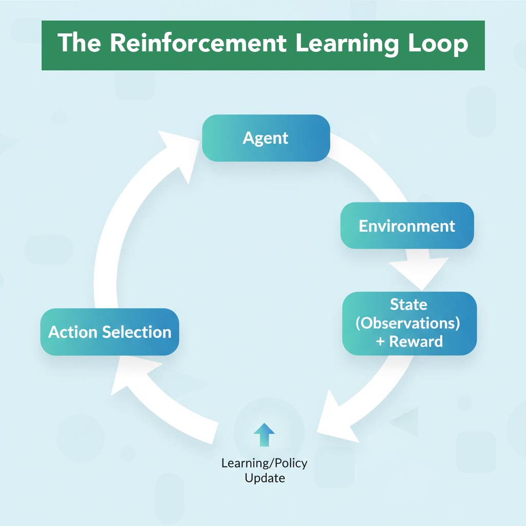
The RL Loop:

1. Agent observes State (S_t)
2. Agent selects Action (A_t) based on current Policy
3. Environment transitions to new State (S_t+1)
4. Agent receives Reward (R_t)
5. Agent updates Policy to maximize future rewards
6. Repeat from step 1

2. Exploration vs. Exploitation

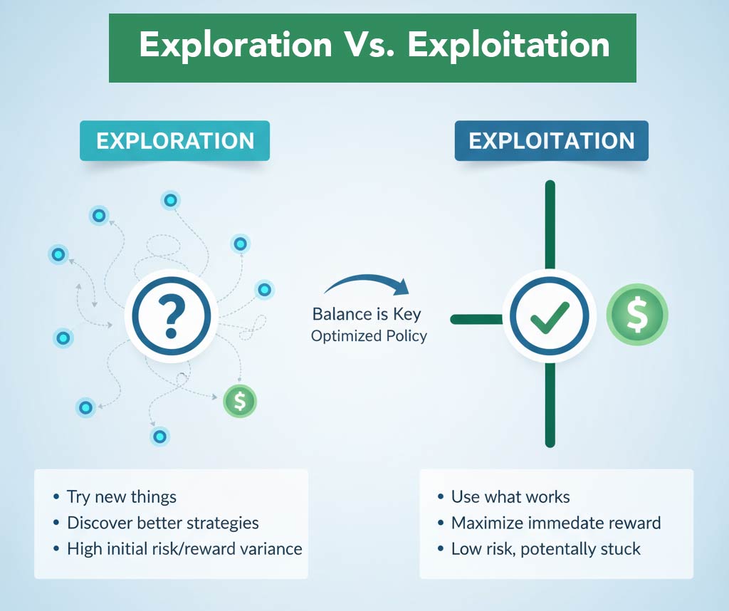
The fundamental RL dilemma:

Exploitation: Use what you know works (current best strategy)
Exploration: Try new things to discover potentially better strategies

Too much exploitation = Agent gets stuck in local optimum (mediocre strategy)
Too much exploration = Agent never settles on a good strategy, keeps trying random things

In trading context:

• Exploitation: Trade the setups you know work
• Exploration: Try marginal setups, different timeframes, new patterns

Good RL agents balance both. Early in training, explore more. Later, exploit more.

3. Value Functions

RL agents learn to estimate the “value” of states and actions:

State Value Function V(s):

• Expected future reward starting from state s
• “How good is this situation?”
• Example: “Being long at VWAP with strong trend = high value”

Action Value Function Q(s, a):

• Expected future reward of taking action a in state s
• “How good is this action in this situation?”
• Example: “Holding this position through 2D target = high Q-value”

Agents learn these value functions through training, then use them to choose actions.

4. Policy Types

Deterministic Policy:

• State → Single action
• “Always buy when RSI < 30”
• Simpler but less flexible

Stochastic Policy:

• State → Probability distribution over actions
• “Buy with 70% probability, hold with 30% when RSI < 30”
• More flexible, better for exploration

5. On-Policy vs. Off-Policy

On-Policy:

• Agent learns from actions it actually takes
• Example algorithms: A2C, PPO
• More stable, safer
• Requires more fresh experience

Off-Policy:

• Agent can learn from past experiences or other agents
• Example algorithms: DQN, SAC, TD3
• More sample-efficient
• Can use replay buffers of old data
• Less stable, more complex

For trading, off-policy is usually better (can learn from historical data).

6. Discount Factor (γ)

How much does the agent value future rewards vs. immediate ones?

• γ = 0: Only care about immediate reward (myopic)
• γ = 0.9: Value future rewards at 90% of immediate
• γ = 0.99: Long-term oriented
• γ = 1.0: All rewards equally important (can be unstable)

In trading:

• Day trading: γ = 0.9 – 0.95 (care about today’s P&L)
• Swing trading: γ = 0.95 – 0.99 (care about week’s performance)
• Position trading: γ = 0.99+ (care about long-term growth)

7. Reward Shaping

Designing the reward function is the most critical (and difficult) part of RL trading.

Bad reward: reward = 1 if profit else -1

• Too sparse, agent doesn’t learn much
• Doesn’t distinguish small vs. large wins

Better reward: reward = realized_PnL

• Direct feedback on profit/loss
• But might encourage high-risk gambling

Even better:

reward = realized_PnL - 0.1 * max_drawdown - 0.01 * trade_count

• Encourages profit
• Penalizes drawdowns
• Discourages overtrading

Best (example):
# Reward based on risk-adjusted returns
sharpe_contribution = (return / volatility) if volatility > 0 else 0
drawdown_penalty = -abs(current_drawdown) * 0.5
reward = sharpe_contribution + drawdown_penalty

Your reward function encodes what you want the agent to optimize for.

---

The RL Trading Framework

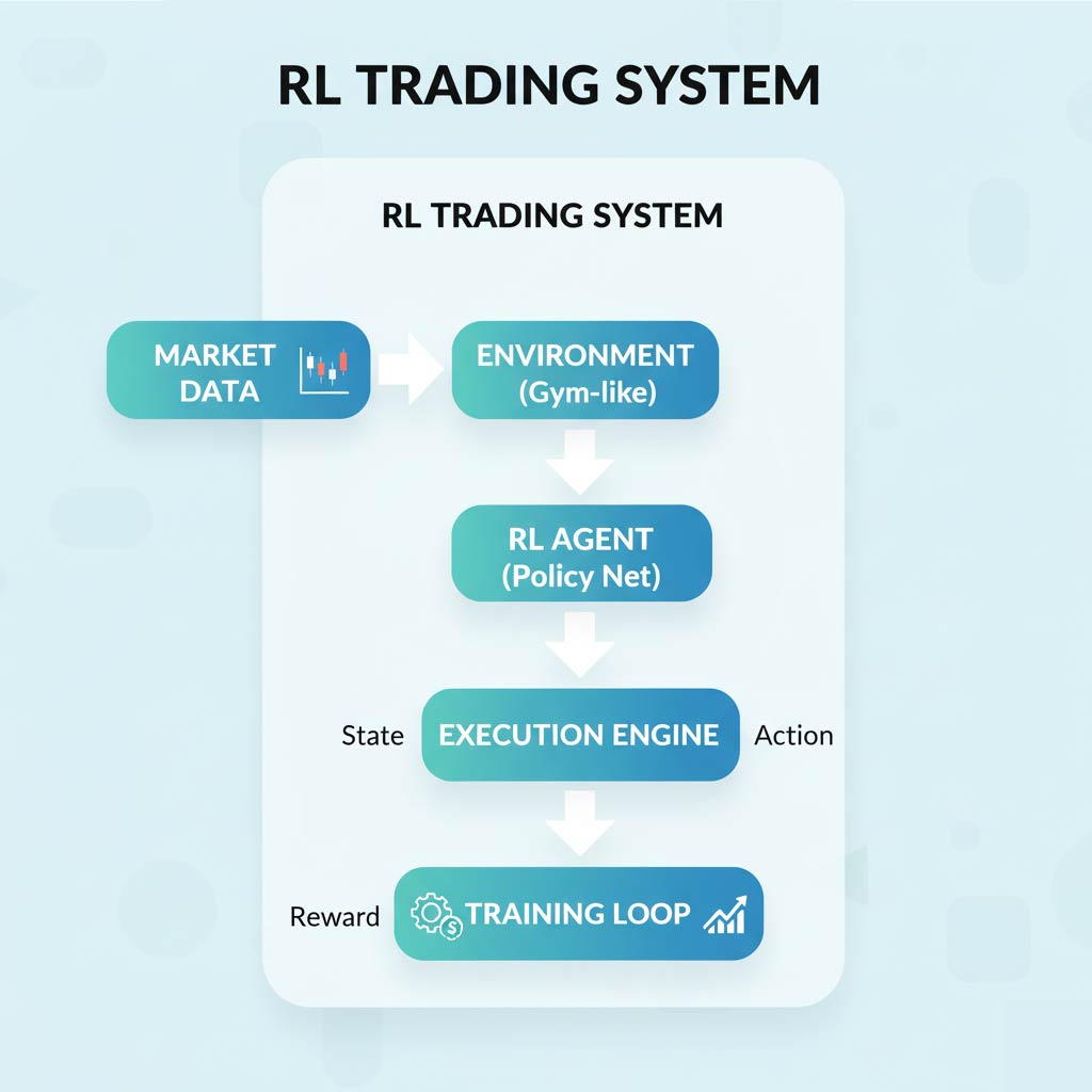
High-Level Architecture

┌─────────────────────────────────────────────────────────┐
│                    RL TRADING SYSTEM                     │
├─────────────────────────────────────────────────────────┤
│                                                          │
│  ┌──────────────┐         ┌───────────────┐             │
│  │   MARKET     │────────▶│  ENVIRONMENT  │             │
│  │   DATA       │         │   (Gym-like)  │             │
│  └──────────────┘         └───────┬───────┘             │
│                                   │                      │
│                                   │ State                │
│                                   ▼                      │
│                           ┌───────────────┐             │
│                           │   RL AGENT    │             │
│                           │  (Policy Net) │             │
│                           └───────┬───────┘             │
│                                   │                      │
│                                   │ Action               │
│                                   ▼                      │
│                           ┌───────────────┐             │
│                           │  EXECUTION    │             │
│                           │   ENGINE      │             │
│                           └───────┬───────┘             │
│                                   │                      │
│                                   │ Reward               │
│                                   ▼                      │
│                           ┌───────────────┐             │
│                           │   TRAINING    │             │
│                           │   LOOP        │             │
│                           └───────────────┘             │
│                                                          │
└─────────────────────────────────────────────────────────┘

Component Breakdown

1. Market Data

• Historical price data (OHLCV bars)
• Real-time feeds (for live trading)
• Technical indicators (calculated from raw data)
• Order flow, volume profile, etc.

2. Environment (Gym-Compatible)

• Manages market simulation
• Tracks agent’s position and P&L
• Calculates rewards
• Handles episode resets
• Enforces trading rules (margin, position limits)

3. RL Agent (The Brain)

• Neural network (or other function approximator)
• Takes state as input
• Outputs action probabilities or Q-values
• Trained to maximize expected cumulative reward

4. Execution Engine

• Translates agent actions into orders
• Manages position sizing
• Handles transaction costs and slippage
• Records trade history

5. Training Loop

• Runs episodes of trading simulation
• Collects experience (state, action, reward, next_state)
• Updates agent’s neural network weights
• Monitors performance metrics
• Saves checkpoints and best models

---

Designing Your Trading Environment

The environment is where your agent “lives” and learns. It must simulate market dynamics realistically while being computationally efficient.

Environment Responsibilities

1. State Representation

What information does the agent see?

Minimal state (simple):

state = [
    normalized_price,      # Current price / recent average
    position,              # -1 (short), 0 (flat), +1 (long)
    unrealized_pnl         # Current position P&L
]

Realistic state (better):

state = [
    # Price features
    normalized_close[-20:],     # Last 20 closes
    normalized_volume[-20:],    # Last 20 volumes
    
    # Technical indicators
    rsi,
    macd_line, macd_signal,
    atr,
    
    # Position info
    position_size,
    entry_price,
    bars_in_trade,
    unrealized_pnl,
    
    # Risk metrics
    current_drawdown,
    account_equity,
    
    # Time features
    time_of_day,
    day_of_week
]

Advanced state (pro):

state = [
    # All above, plus:
    order_flow_imbalance,
    vwap_deviation,
    volume_profile_poc,
    institutional_h_levels,    # Your proprietary edge
    multi_timeframe_srsi,
    session_type,              # Asian/European/US
]

Key principle: Include only information you believe is predictive. More isn’t always better (curse of dimensionality).

2. Action Space

What can the agent do?

Discrete actions (simpler):

actions = {
    0: 'hold',
    1: 'buy',
    2: 'sell'
}

Continuous actions (advanced):

action = [
    position_change,    # -1.0 to +1.0 (short to long)
    stop_distance,      # 0.0 to 1.0 (% of ATR)
]

Multi-discrete (most flexible):

action = [
    direction,     # 0=flat, 1=long, 2=short
    size,          # 0=none, 1=half, 2=full
    stop_type,     # 0=none, 1=fixed, 2=trailing
]

For beginners: Start with simple discrete (buy/sell/hold).

3. Reward Function Design

This is where art meets science.

Simple but flawed:

reward = current_equity - previous_equity

Problems:

• Encourages gambling (big bets for big rewards)
• No penalty for risk
• Doesn’t account for drawdowns

Better (risk-adjusted):

if trade_closed:
    reward = (exit_price - entry_price) / atr  # R-multiple
else:
    reward = -0.001  # Small penalty for time in market

Even better (comprehensive):

# Realized profit/loss
pnl_reward = realized_pnl * 0.01

# Sharpe ratio contribution
returns = pnl_reward / account_equity
sharpe_reward = returns / recent_volatility if recent_volatility > 0 else 0

# Drawdown penalty
dd_penalty = -abs(current_drawdown / max_equity) * 0.5

# Trade count penalty (discourage overtrading)
trade_penalty = -0.001 if new_trade else 0

# Final reward
reward = pnl_reward + sharpe_reward + dd_penalty + trade_penalty

Pro tips:

• Normalize rewards to roughly -1 to +1 range
• Use sparse rewards (only at trade exit) initially, then add dense shaping if needed
• Penalize bad behavior (excessive drawdown, overtrading)
• Reward good process, not just outcomes

4. Episode Management

When does a training episode start/end?

Fixed length episodes:

episode_length = 1000 bars  # ~1 week of 5-min data
reset after 1000 steps

Pros: Predictable, stable
Cons: Doesn’t teach agent to manage positions over different horizons

Variable length episodes:

reset when:
- Account blown up (equity < 50%)
- Large drawdown (> 20%)
- Maximum time reached (5000 bars)

Pros: More realistic
Cons: Less stable, harder to tune

Rolling window episodes:

randomly sample start point in historical data
run for fixed length from there

Pros: Exposes agent to many market conditions
Cons: Can be computationally expensive

5. Transaction Costs & Slippage

Critical: Don’t forget these, or your agent will learn strategies that can’t work live.

# On every trade execution
slippage = 0.0001 * price  # 1 tick
commission = 2.50          # Per contract
realized_pnl -= (slippage + commission)

Be conservative. Real slippage is worse than you think, especially in volatile markets.

6. Position Sizing & Risk Management

Should the environment handle this, or the agent?

Option 1: Agent controls size

• Agent outputs position size as part of action
• More flexible, can learn position sizing
• Harder to train, more complex

Option 2: Environment enforces fixed size

• Agent only chooses direction (long/short/flat)
• Environment applies consistent position sizing rules
• Simpler, more stable
• Less flexible

For beginners: Start with Option 2.

# Environment enforces 1% risk per trade
position_size = (account_equity * 0.01) / (stop_distance * tick_value)

---

Choosing Your RL Algorithm

Not all RL algorithms are suitable for trading. Here’s a practical guide:

Algorithm Categories

1. Value-Based Methods

Learn Q(s, a) = expected future reward of action a in state s

DQN (Deep Q-Network):

• Pros: Well-established, works for discrete actions, sample-efficient
• Cons: Only discrete actions, can be unstable
• Best for: Simple buy/sell/hold strategies

Double DQN / Dueling DQN:

• Improvements on DQN addressing overestimation and value/advantage separation
• Best for: Same as DQN but more stable

2. Policy-Based Methods

Learn π(a|s) = probability of action a given state s

REINFORCE:

• Pros: Simple, works with continuous actions
• Cons: High variance, sample-inefficient, slow to train
• Best for: Educational purposes, not production

A2C (Advantage Actor-Critic):

• Pros: Lower variance than REINFORCE, on-policy, stable
• Cons: Sample-inefficient, requires many environment interactions
• Best for: When you have fast simulation and want stability

PPO (Proximal Policy Optimization):

• Pros: Very stable, good default choice, widely used in industry
• Cons: On-policy (can’t use old data efficiently)
• Best for: Most trading applications, especially when starting

3. Actor-Critic Methods

Combine value and policy learning

SAC (Soft Actor-Critic):

• Pros: Off-policy, sample-efficient, handles continuous actions, very stable
• Cons: More complex, harder to tune
• Best for: Advanced traders, continuous action spaces (position sizing)

TD3 (Twin Delayed DDPG):

• Pros: Off-policy, continuous actions, stable
• Cons: Complex, many hyperparameters
• Best for: When SAC is overkill but you need continuous actions

Recommendation for Trading

Beginner:
→ PPO with discrete actions (Buy/Sell/Hold)

Why:

• Stable and forgiving
• Good documentation and community support
• Works well with Stable-Baselines3 library
• Easy to understand and debug

Intermediate:
→ SAC with continuous actions

Why:

• More sample-efficient (can reuse old data)
• Handles complex action spaces (position sizing, stop placement)
• State-of-the-art performance

Advanced:
→ Custom hybrid approach

Why:

• Combine RL agent with rule-based risk management
• Multi-agent systems (different agents for different market regimes)
• Ensemble methods

Popular Libraries

Stable-Baselines3 (Recommended)

pip install stable-baselines3

• Clean API, good documentation
• Implements PPO, A2C, SAC, TD3, DQN
• Easy to get started
• Built on PyTorch

RLlib (Ray)

pip install ray[rllib]

• Scalable distributed training
• Many algorithms implemented
• Production-ready infrastructure
• Steeper learning curve

TensorFlow Agents

pip install tf-agents

• Built on TensorFlow
• Good for TensorFlow users
• Less popular than SB3

Recommendation: Start with Stable-Baselines3. It has the best balance of power and ease of use.

---

The Training Process

Step-by-Step Training Workflow

1. Data Preparation

# Load historical data
import pandas as pd

data = pd.read_csv('ES_5min_2020-2025.csv')

# Calculate technical indicators
data['rsi'] = calculate_rsi(data['close'], period=14)
data['atr'] = calculate_atr(data, period=14)
# ... more features

# Split data
train_data = data['2020':'2023']  # 3 years training
val_data = data['2024':'2024']    # 1 year validation
test_data = data['2025':'2025']   # Out-of-sample test

2. Environment Setup

from trading_env import TradingEnv

# Create environment
env = TradingEnv(
    data=train_data,
    initial_balance=100000,
    commission=2.50,
    slippage_pct=0.0001
)

# Verify environment
from stable_baselines3.common.env_checker import check_env
check_env(env)  # Ensures environment is compatible

3. Model Initialization

from stable_baselines3 import PPO

# Create RL agent
model = PPO(
    policy='MlpPolicy',         # Multi-layer perceptron
    env=env,
    learning_rate=3e-4,
    n_steps=2048,               # Steps before update
    batch_size=64,
    n_epochs=10,
    gamma=0.99,                 # Discount factor
    verbose=1,
    tensorboard_log='./logs/'
)

4. Training Loop

# Train for 1 million steps
total_timesteps = 1_000_000

model.learn(
    total_timesteps=total_timesteps,
    callback=callbacks,  # For monitoring and checkpoints
)

# Save trained model
model.save('ppo_trading_agent')

5. Monitoring During Training

Use TensorBoard to track:

• Episode rewards (trending up = learning)
• Episode length (should stabilize)
• Policy loss (should decrease)
• Value loss (should decrease)
• Explained variance (higher = better value function)

tensorboard --logdir ./logs/

6. Validation

# Load validation environment
val_env = TradingEnv(data=val_data, initial_balance=100000)

# Test agent
obs = val_env.reset()
done = False
total_reward = 0

while not done:
    action, _ = model.predict(obs, deterministic=True)
    obs, reward, done, info = val_env.step(action)
    total_reward += reward

print(f'Validation Reward: {total_reward}')

7. Hyperparameter Tuning

If validation performance is poor, try adjusting:

• Learning rate (lower if unstable, higher if slow)
• Network architecture (deeper/wider for complex patterns)
• Reward function (most impactful change)
• State features (add/remove based on importance)
• Discount factor γ (higher for longer-term strategies)

8. Final Evaluation (Out-of-Sample)

# Test on unseen 2025 data
test_env = TradingEnv(data=test_data, initial_balance=100000)

# Run test
results = evaluate_agent(model, test_env, n_episodes=10)

print(f'Test Win Rate: {results["win_rate"]}')
print(f'Test Sharpe: {results["sharpe"]}')
print(f'Test Max DD: {results["max_drawdown"]}')

Only if test results are good should you consider live trading.

Training Time Expectations

CPU Training:

• 1M timesteps: 2-6 hours (depending on environment complexity)
• 10M timesteps: 20-60 hours

GPU Training:

• Minimal benefit for small networks (PPO with MLP)
• Useful for larger networks or image-based states

Cloud Training:

• AWS EC2 (c5.4xlarge): ~$0.68/hour
• Google Colab Pro: $10/month, faster GPUs
• Can train 10M timesteps overnight

Common Training Issues

1. Agent Not Learning (Flat Reward)

Possible causes:

• Reward signal too sparse
• State doesn’t contain enough information
• Learning rate too low
• Environment too difficult

Solutions:

• Add reward shaping
• Include more predictive features in state
• Increase learning rate
• Simplify environment initially

2. Training Unstable (Reward Oscillates Wildly)

Possible causes:

• Learning rate too high
• Reward function not normalized
• Network architecture too large
• Exploration too aggressive

Solutions:

• Decrease learning rate
• Normalize rewards to -1 to +1 range
• Use smaller network
• Decrease epsilon (if using epsilon-greedy)

3. Agent Overfits Training Data

Symptoms:

• Great training performance
• Terrible validation performance

Solutions:

• Use more diverse training data
• Add regularization (dropout, L2)
• Simplify model architecture
• Train for fewer steps

4. Agent Learns Degenerate Strategy

Example: Agent learns to never trade (always holds)

Causes:

• Reward function poorly designed
• Action penalties too harsh
• Risk-free rate too attractive

Solutions:

• Adjust reward to encourage trading when appropriate
• Reduce penalties for losses
• Add reward for taking actions

---

Evaluation and Validation

Key Metrics for Trading Agents

1. Profitability Metrics

Total Return:

total_return = (final_equity - initial_equity) / initial_equity

Sharpe Ratio: (Most important for professional trading)

sharpe = (mean_returns - risk_free_rate) / std_returns * sqrt(252)

Target: > 1.5 (good), > 2.0 (excellent)

Sortino Ratio: (Penalizes only downside volatility)

sortino = (mean_returns - risk_free_rate) / downside_std * sqrt(252)

2. Risk Metrics

Maximum Drawdown:

drawdown = (peak_equity - current_equity) / peak_equity
max_drawdown = max(all_drawdowns)

Target: < 20% (good), < 10% (excellent)

Win Rate:

win_rate = winning_trades / total_trades

Not as important as R:R, but psychologically significant

Risk-Reward Ratio:

avg_win = sum(winning_trades) / num_wins
avg_loss = sum(losing_trades) / num_losses
r_r_ratio = avg_win / abs(avg_loss)

Target: > 1.5

3. Behavioral Metrics

Trade Frequency:

• Too high = overtrading, likely losing to commissions
• Too low = agent not finding opportunities

Average Trade Duration:

• Should align with your strategy type (scalp vs. swing)

Consecutive Losses:

• Track maximum consecutive losing streak
• Important for psychological resilience

Backtesting vs. Walk-Forward Analysis

Backtesting (Necessary but insufficient):

# Train on 2020-2023, test on 2024
# Problem: 2024 data is just one market regime

Walk-Forward Analysis (Better):

# Train on 2020-2021, test on 2022
# Retrain on 2020-2022, test on 2023
# Retrain on 2020-2023, test on 2024
# Multiple out-of-sample periods = more robust

Monte Carlo Simulation (Best for robustness):

# Randomly shuffle trade outcomes
# Run 1000 simulations
# Check: What % of simulations are profitable?
# If < 95%, strategy might be luck

Comparing Agent to Baselines

Always compare your RL agent to simple baselines:

Baseline 1: Buy and Hold

# Just buy at start, hold entire period
# Hard to beat in bull markets

Baseline 2: Random Agent

# Take random actions
# Your agent should beat this easily

Baseline 3: Simple Rule-Based Strategy

# Example: Buy when RSI < 30, sell when RSI > 70
# If your RL agent can't beat this, it's not learning anything useful

Baseline 4: Supervised Learning (if applicable)

# Train classifier to predict up/down
# Trade based on predictions
# RL should beat this by considering sequences

If your RL agent doesn’t outperform all baselines, something is wrong.

Statistical Significance Testing

Don’t trust single backtest results. Use statistical tests:

Bootstrap Resampling:

# Resample your trades with replacement
# Compute Sharpe ratio for each bootstrap sample
# Check 95% confidence interval
# If it includes zero, not statistically significant

Permutation Test:

# Shuffle trade outcomes randomly
# Compute Sharpe ratio for shuffled trades
# Repeat 1000 times
# p-value = % of shuffles that beat actual Sharpe
# If p < 0.05, results are significant

---

Common Pitfalls and How to Avoid Them

Pitfall 1: Look-Ahead Bias

Mistake: Using information from the future in your state

Example:

# WRONG: Using close price of current bar before bar completes
state = [current_bar_close, rsi, macd]
# Agent sees close price, makes decision, then close price is revealed
# This is impossible in live trading

Solution:

# RIGHT: Use only information available at decision time
state = [previous_bar_close, rsi_calculated_from_previous_bars, ...]
# Agent makes decision, then sees how current bar closes

Test: Paper trade your agent with real-time data. If performance drops dramatically, you have look-ahead bias.

Pitfall 2: Overfitting to Historical Data

Mistake: Training too long or on too little data diversity

Symptoms:

• 90% win rate in backtest
• 30% win rate in live trading

Solution:

• Use walk-forward analysis
• Train on multiple market regimes (trending, ranging, volatile)
• Keep model simple (fewer parameters)
• Regularization (dropout, early stopping)
• Out-of-sample testing before live

Pitfall 3: Ignoring Transaction Costs

Mistake: Not modeling slippage and commissions

Result: Agent learns high-frequency strategy that loses money to costs

Solution:

# Be conservative with cost estimates
commission = 2.50 per contract (futures)
slippage = 0.0002 * price (2 ticks)
# Apply on EVERY trade in simulation

Pitfall 4: Reward Hacking

Mistake: Poorly designed reward function leads to unintended behavior

Example:

# WRONG: Reward = equity
# Problem: Agent learns to maximize equity by taking huge risks
# Works until it doesn't (then blows up)

Solution:

# RIGHT: Reward = risk-adjusted return
reward = pnl / max_drawdown
# Encourages profit while penalizing risk

Pitfall 5: Data Leakage

Mistake: Using test data during training or validation

Example:

# WRONG:
scaler.fit(entire_dataset)
train_data = scaler.transform(train_split)
test_data = scaler.transform(test_split)
# Scaler learned statistics from test set!

Solution:

# RIGHT:
scaler.fit(train_split)
train_data = scaler.transform(train_split)
test_data = scaler.transform(test_split)
# Scaler only learned from training data

Pitfall 6: Insufficient Training Data

Mistake: Training on 6 months of data, expecting it to work forever

Markets evolve. Agents need exposure to diverse conditions:

• Bull markets and bear markets
• High volatility and low volatility
• Trending and ranging
• Different seasons and regime changes

Solution:

• Train on 3-5 years minimum
• Include multiple market cycles
• Walk-forward validate across different periods

Pitfall 7: Not Testing Edge Cases

Mistake: Only testing in “normal” market conditions

What happens when:

• Market gaps overnight?
• Flash crash occurs?
• Liquidity dries up?
• Data feed goes down?

Solution:

• Stress test your agent
• Simulate edge cases explicitly
• Add safeguards (max position size, kill switch)

Pitfall 8: Complexity Creep

Mistake: Adding more and more features/complexity hoping it helps

Result:

• Overfitting increases
• Training becomes unstable
• Model is impossible to debug

Solution:

• Start simple (3-5 state features)
• Add complexity only when simple doesn’t work
• Remove features that don’t improve validation performance
• Ablation studies (remove one feature at a time, see impact)

---

Path to Production

Going from trained agent to live trading requires careful planning.

Pre-Production Checklist

1. Statistical Validation ✓

• Agent beats all baselines in out-of-sample testing
• Sharpe ratio > 1.5 on test set
• Results are statistically significant (p < 0.05)
• Walk-forward analysis shows consistency
• Monte Carlo simulations 95%+ positive

2. Paper Trading ✓

• Run agent in paper trading for 1-3 months
• Performance matches backtest expectations
• No implementation bugs discovered
• All edge cases handled correctly
• Latency and execution quality acceptable

3. Risk Management ✓

• Position sizing limits enforced
• Maximum daily loss limit set
• Maximum drawdown kill switch implemented
• Emergency shutdown procedures documented
• Backup plan if agent fails

4. Infrastructure ✓

• Execution system tested and reliable
• Data feed redundancy in place
• Monitoring and alerts configured
• Logging comprehensive
• Able to review and debug any trade

5. Mental Preparation ✓

• Comfortable with expected drawdowns
• Understand agent’s strategy and logic
• Willing to shut down if something’s wrong
• Have contingency plan for failures
• Not betting money you can’t afford to lose

Live Deployment Strategy

Phase 1: Micro Position Sizes (Week 1-4)

• Start with 10% of target position size
• Goal: Validate execution, not make money
• Watch for ANY unexpected behavior
• Log everything, review daily

Phase 2: Quarter Position Sizes (Week 5-8)

• If Phase 1 went well, increase to 25% size
• Still in “validation” mode
• Performance should track paper trading
• No major surprises

Phase 3: Half Position Sizes (Week 9-12)

• Increase to 50% of target size
• Starting to matter financially
• Agent should be performing as expected
• Confidence building

Phase 4: Full Position Sizes (Month 4+)

• Only if everything has gone smoothly
• Full-scale deployment
• Continuous monitoring still required
• Regular performance reviews

Ongoing Monitoring

Even in production, never “set and forget”:

Daily:

• Review agent’s trades
• Check for any unusual behavior
• Verify P&L matches expectations
• Monitor for system errors

Weekly:

• Compare live results to backtest expectations
• Calculate rolling Sharpe ratio
• Check if edge is degrading
• Review largest winners and losers

Monthly:

• Full performance analysis
• Decide: Continue, adjust, or shut down
• Consider retraining if market regime changed
• Document learnings

Quarterly:

• Walk-forward retraining (if appropriate)
• Update risk parameters based on realized volatility
• Review and improve based on 3 months data

When to Shut Down the Agent

Immediate shutdown if:

• Single loss exceeds max loss limit (bug or extreme event)
• Agent starts taking nonsensical actions
• System error that compromises execution
• Sharpe ratio drops to negative over 2 weeks

Pause and review if:

• Drawdown exceeds expected from backtests
• Win rate drops significantly
• Agent’s behavior changes unexpectedly
• Performance lags backtests for 1 month

It’s okay to shut down! Better to stop and reassess than to lose money stubbornly hoping the agent will “figure it out.”

Continuous Improvement

RL agents are not “done” once deployed:

• Version 1.0: Initial deployment
• Version 1.1: Fix bugs discovered in live trading
• Version 1.2: Add features based on live learnings
• Version 2.0: Retrain with updated reward function
• Version 3.0: Completely new architecture based on 1 year of data

Treat your agent as a living system that evolves.

---

Resources and Next Steps

Learning Path

If you’re brand new to RL:

1. Learn RL fundamentals:
   • Course: David Silver’s RL Course (free)
   • Book: Reinforcement Learning: An Introduction by Sutton & Barto (free PDF)
2. Get hands-on with OpenAI Gym:
   • Tutorial: Stable-Baselines3 Getting Started
   • Practice: Solve CartPole, MountainCar, LunarLander
3. Learn trading basics:
   • Understand market mechanics (order types, liquidity, slippage)
   • Learn technical analysis (indicators, chart patterns)
   • Study position sizing and risk management
4. Combine RL + Trading:
   • Start with simple Gym trading environments (from GitHub)
   • Build your own environment with real data
   • Train your first agent
   • Iterate and improve

If you’re experienced in RL but new to trading:

1. Learn trading first:
   • Paper trade manually for 3-6 months
   • Understand why strategies work or fail
   • Learn market microstructure
2. Build simple rule-based systems:
   • Moving average crossovers
   • Mean reversion strategies
   • Trend following
3. Then apply RL:
   • Your domain knowledge will guide state/action design
   • You’ll recognize when agent learns something sensible
   • You’ll avoid common trading mistakes

If you’re experienced in trading but new to RL:

1. Learn RL fundamentals (see above)
2. Start with supervised learning:
   • Build price prediction models
   • Understand model training and validation
   • Get comfortable with ML workflows
3. Move to RL:
   • Your trading knowledge is your edge
   • Focus on reward function design
   • Encode your expertise into the environment

Key Resources

Libraries & Frameworks:

• Stable-Baselines3 – Best RL library for beginners
• FinRL – Trading-specific RL framework
• OpenAI Gym – Standard RL environment interface
• QuantConnect – Backtesting platform with data

Papers:

• Deep Reinforcement Learning for Trading by Théate & Ernst (2021)
• Practical Deep Reinforcement Learning Approach for Stock Trading by Xiong et al. (2018)

Communities:

• r/algotrading – Reddit community for algo traders
• r/reinforcementlearning – RL discussions
• QuantConnect forums – Systematic trading community

Data Sources:

• Alpha Vantage – Free API for stocks
• IEX Cloud – Market data API
• Polygon.io – Real-time and historical data
• Yahoo Finance – Free historical data

Books:

• Advances in Financial Machine Learning by Marcos López de Prado
• Quantitative Trading by Ernest Chan
• Reinforcement Learning by Sutton & Barto
• Artificial Intelligence for Trading by Tucker Balch

Next Steps

Your action plan:

Week 1-2: Fundamentals

• Complete David Silver RL lectures (or similar)
• Read Sutton & Barto chapters 1-6
• Install Stable-Baselines3 and solve CartPole

Week 3-4: Simple Trading Env

• Download historical price data (1 instrument, 1 year)
• Build basic Gym environment (buy/sell/hold, simple state)
• Train PPO agent
• Evaluate performance

Week 5-8: Iterate and Improve

• Add technical indicators to state
• Experiment with reward functions
• Try different algorithms (SAC, A2C)
• Walk-forward testing

Week 9-12: Realistic Environment

• Add transaction costs and slippage
• More complex state (multi-timeframe, more features)
• Implement proper position sizing
• Paper trade best agent

Month 4-6: Validation

• Test on multiple instruments
• Statistical significance testing
• Compare to baselines
• If promising: prepare for micro live trading

Month 7+: Production (Maybe)

• Only if validation results are excellent
• Start with tiny position sizes
• Monitor obsessively
• Iterate based on live learnings

Final Advice

Building a profitable trading RL agent is a marathon, not a sprint.

Most will fail. That’s okay—the learning is valuable regardless.

Keys to success:

1. Start simple. Complexity comes later.
2. Validate rigorously. Don’t trust single backtests.
3. Learn trading first. RL can’t fix a bad strategy.
4. Be patient. 6-12 months is realistic timeline.
5. Manage risk. Never risk more than you can afford to lose.
6. Stay humble. Markets are humbling; RL agents even more so.

You don’t need to build the perfect agent on your first try.

Build something simple that works. Then improve it. Then improve it again.

Version 1.0 doesn’t have to be perfect. It just has to teach you what Version 2.0 should be.

---

Conclusion

Reinforcement learning for trading is one of the most challenging applications of machine learning. It combines the complexity of financial markets with the difficulty of RL algorithms.

But it’s also one of the most rewarding (literally and intellectually).

When you finally train an agent that discovers a profitable strategy you didn’t explicitly program, it’s genuinely magical. The agent learned to trade through pure interaction with data, finding patterns and strategies you might never have considered.

This guide gave you the conceptual foundation:

• What RL agents are and how they work
• Why RL is (and isn’t) suited for trading
• Core RL concepts you need to understand
• How to design a trading environment
• Which algorithms to use
• How to train, validate, and deploy
• Common pitfalls and how to avoid them

The next step is building.

Start small. Build a simple environment. Train your first agent. It will probably lose money. That’s fine—you’ll learn why, fix it, and try again.

Each iteration teaches you something:

• About RL algorithms
• About market dynamics
• About system design
• About yourself as a trader

Some will build agents that make money. Most won’t. But everyone who tries seriously will learn skills that are valuable across ML, trading, and system design.

Good luck. Build responsibly. Trade carefully.

And remember: the goal isn’t just to make money—it’s to understand how markets work deeply enough that you can teach a computer to trade them.

That understanding is the real prize.

---

Tyler Archer
Systematic Trader & ML Researcher
November 2025

---

Appendix: Glossary

Action: Decision the agent makes (buy, sell, hold)

Agent: The RL algorithm that learns to trade

Environment: Simulated market where agent practices

Episode: One complete trading session from start to reset

Exploration: Trying new actions to discover better strategies

Exploitation: Using known good strategies

Gym: OpenAI’s standard RL environment interface

Policy (π): Agent’s strategy (state → action mapping)

Reward: Feedback signal (profit/loss, risk-adjusted return)

State: Agent’s observation of the market

Timestep: One increment in the simulation (e.g., one 5-min bar)

Value Function: Expected future reward from a state

Q-Value: Expected future reward from taking action in state

MDP: Markov Decision Process (formal RL framework)

On-policy: Agent learns from actions it takes

Off-policy: Agent can learn from old data or other agents

Discount Factor (γ): How much agent values future vs. immediate rewards

Actor-Critic: RL approach combining policy (actor) and value (critic)

PPO: Proximal Policy Optimization (popular RL algorithm)

SAC: Soft Actor-Critic (advanced RL algorithm)

DQN: Deep Q-Network (value-based RL algorithm)

Stable-Baselines3: Popular RL library in Python

OpenAI Gym: Standard interface for RL environments

Sharpe Ratio: Risk-adjusted return metric (higher is better)

Drawdown: Peak-to-trough decline in equity

Overfitting: Agent works on training data but fails on new data

Backtest: Testing strategy on historical data

Walk-forward: Sequential out-of-sample testing method

Paper Trading: Simulated live trading with fake money

Look-ahead Bias: Using future information in backtests (error)

Slippage: Difference between expected and actual execution price